
Reinforcement Learning (RL) stands as a powerful paradigm for creating intelligent agents capable of autonomous decision-making in complex, dynamic environments. This comprehensive guide delves into the foundational concepts of RL, starting with the essential agent-environment interaction and progressing to the mathematical rigor of Markov Decision Processes (MDPs). We will explore how agents define strategies through policies and quantify future rewards with value functions, culminating in a detailed look at classic control algorithms like Policy and Value Iteration that drive optimal behavior.
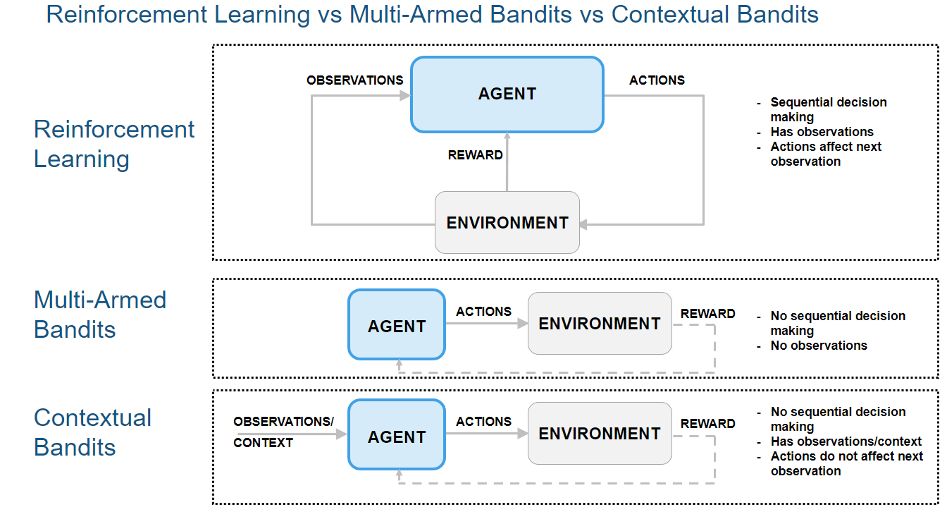
At the heart of any Reinforcement Learning system lies a fundamental, continuous interaction loop between two primary entities: the Agent and its Environment. The agent serves as the learner and decision-maker, actively selecting and executing an action at each step. This chosen action directly influences the environment, causing it to transition from its current configuration to a new state. Crucially, in response to the agent's action and the resulting state change, the environment provides vital feedback back to the agent, thereby completing the cycle. This iterative process of observation, action, and feedback is the bedrock upon which the agent's learning process is built.
The feedback provided by the environment to the agent manifests primarily in two critical forms: States and Rewards.
A State precisely describes the current configuration or condition of the environment. It provides the agent with all the necessary contextual information to make an informed decision at that particular moment. The state encapsulates the relevant aspects of the environment that the agent perceives.
An Action represents the specific operation, decision, or control signal that the agent performs within a given state. These actions are the agent's means of influencing the environment and progressing through its task.
Following an action, the environment issues a Reward. This is a scalar numerical value that quantifies the immediate desirability or undesirability of the agent's action and the resulting transition to a new state. A positive reward indicates a favorable outcome, while a negative reward (often termed a penalty) signifies an unfavorable one.
The overarching goal of the agent is not merely to maximize immediate rewards, but rather to maximize the cumulative reward over the long term. Through this iterative cycle of observing states, performing actions, and receiving rewards, the agent progressively learns which sequences of actions lead to the most favorable long-term outcomes, thereby discovering an optimal policy for navigating its environment.
Sequential decision-making under uncertainty is a fundamental aspect of Reinforcement Learning. The Multi-Arm Bandit (MAB) problem serves as an accessible entry point to this domain, illustrating core concepts before progressing to more complex frameworks that address more intricate challenges.
The Multi-Arm Bandit (MAB) problem models a decision-maker faced with a finite set of choices, often referred to as "arms," each yielding a reward drawn from an unknown probability distribution. Analogous to a gambler selecting from multiple slot machines, where each machine (arm) has a distinct, unknown payout probability, the objective is to maximize the total cumulative rewards over a series of independent decisions.

The central challenge in MAB is the exploration-exploitation trade-off. Exploitation involves consistently choosing the arm that has historically provided the highest average reward, aiming for immediate gains based on current knowledge. Conversely, exploration entails trying less-chosen or untried arms to gather more information about their true reward distributions, with the potential of discovering a more lucrative long-term payout. This dilemma is inherent in scenarios where optimizing immediate reward competes with acquiring knowledge for future benefit. A key characteristic of the MAB problem is the assumption of a single, independent decision at each time step, where the environment does not change based on past actions, and there is no sequence of interconnected states. The reward received from pulling an arm does not influence the availability or characteristics of other arms or future states.
Building upon the MAB framework, the Contextual Multi-Arm Bandit (C-MAB) problem introduces "context" or "state information" into the decision process. Unlike traditional MABs where rewards are independent of external factors, in a C-MAB, the optimal action (arm selection) is contingent on the current situation or observable features of the environment. For instance, when recommending an article to a user, the most suitable article (arm) may vary based on the user's browsing history, demographics, or the current time of day—this constitutes the context. The agent observes this context before making a decision at each step.
This integration of state information renders the problem more realistic and powerful, as decisions are no longer isolated but are informed by the environment's current state. The objective in a C-MAB is to learn a policy that maps observed contexts to optimal actions, thereby maximizing cumulative reward. This fundamental difference means that while MAB assumes a static optimal arm (or set of arms) regardless of the situation, C-MAB acknowledges that the best action depends dynamically on the current context.
While MAB and C-MAB problems are valuable for understanding the exploration-exploitation trade-off and the role of context in decision-making, they present significant simplifications regarding temporal dynamics. They primarily focus on single-step or short-horizon decisions where the immediate reward is the primary concern. Bandit frameworks are insufficient for scenarios where an agent's actions have long-term consequences, and the environment dynamically evolves over time as a result of those actions.
Bandit problems have certain limitations in their modeling approach:
Lack of Influence on Future States: Actions taken in the present do not impact future states or decision opportunities.
No State Transition or Delayed Reward: Traditional bandit formulations do not incorporate the concepts of state transitions or delayed rewards.
Static Environment: The environment’s state remains unchanged regardless of the agent’s actions, and future rewards are not influenced by past actions.
For scenarios that demand foresight, planning across interconnected states, and evaluating the long-term effects of current decisions, a more robust mathematical framework is necessary. This is where full Reinforcement Learning comes into play, offering comprehensive tools to address these complexities.
Markov Decision Processes (MDPs) provide a formal mathematical framework for modeling sequential decision-making problems. An MDP is typically characterized by a tuple (S, A, P, R, γ, H) , where each element plays a critical role in defining the problem.
The Discount Factor (γ) is a key parameter in reinforcement learning that quantifies the present value of future rewards. It has a value ranging from 0 to 1 (inclusive) and plays a crucial role in balancing immediate gratification against long-term objectives.
High γ (closer to 1): Emphasizes long-term rewards, encouraging the agent to consider future consequences more heavily.
Low γ (closer to 0): Makes the agent more "myopic," prioritizing immediate rewards over future ones.
The fundamental components of an MDP define the environment and the agent's interaction within it:
States (S) represent all possible configurations or observable conditions of the environment at any given time. While often considered finite for theoretical simplicity and tractability, state spaces can be countably infinite or even continuous in practical applications. In such cases, techniques like function approximation become essential to manage the immense or infinite number of states.
Actions (A) constitute the set of choices available to the agent when in a particular state. These actions are the agent's means of influencing the environment's evolution, leading to new states and potentially new rewards.
The Transition Probability (P) defines the dynamics of the environment, capturing its inherent uncertainty. Specifically, P(s’|s, a) denotes the probability of transitioning to a next state s’ from the current state s after the agent takes action a. This probabilistic nature is fundamental to modeling real-world environments where outcomes are not always deterministic.
The Reward Function (R) provides immediate scalar feedback to the agent, indicating the desirability of a specific state-action-next-state transition. R(s,a,s’) assigns a numerical value representing the immediate reward received by the agent for taking action a in state s and subsequently transitioning to state s’. While rewards can also be stochastic, the primary source of uncertainty in MDPs typically stems from the probabilistic state transitions.
The Horizon (H) specifies the total number of steps or time stages in an episode of the decision-making process. The horizon can be finite, as seen in games with a fixed number of turns, or infinite, which is common in continuous control tasks where the process continues indefinitely until a terminal condition is met or a steady state is achieved.
A critical characteristic that underpins the power and analytical tractability of MDPs is the Markov Property. This property asserts that the future state and the reward depend only on the current state and the action taken, and are conditionally independent of all previous states and actions. Formally, this can be expressed as:
This simplification is profoundly significant because it allows the agent to make optimal decisions based solely on the current state, without needing to recall or process the entire history of interactions. It implies that the current state encapsulates all necessary information from the past to predict the future. For many well-defined MDPs, the optimal policy itself is also Markov, meaning the optimal action in any state depends only on that state. However, it's important to note that for more complex scenarios, such as Partially Observable Markov Decision Processes (POMDPs) where the current state is not fully observable, or Multi-Agent Reinforcement Learning (MARL) where interactions are complex, policies may need to consider historical observations to infer a more complete understanding of the environment.
This formalization of states, actions, transitions, and rewards, rigorously underpinned by the Markov Property, provides a robust mathematical foundation for understanding how agents learn to navigate and optimize their behavior in dynamic and uncertain environments. It enables the development of algorithms that can effectively derive optimal policies for sequential decision-making.
Reinforcement Learning (RL) agents operate within dynamic environments, learning optimal strategies through interaction. Understanding the fundamental concepts of these environments, the agent's strategy (policy), and how future rewards are estimated (value functions) is crucial for grasping how RL systems function. This section delves into these core components, including the critical role of the discount factor.
In Reinforcement Learning, the environment is everything an agent interacts with, providing states, rewards, and determining the consequences of actions. The nature of this environment significantly influences the learning approach. Environments can broadly be categorized based on whether the agent has a complete model of the world or not.
When an agent operates in a known environment, it possesses a complete model of the environment's dynamics—meaning it knows exactly how actions will transition it between states and what rewards will be received. This allows for planning, where the agent can compute optimal strategies offline without direct interaction, often leveraging techniques like dynamic programming.
Conversely, in unknown environments, the agent does not have a complete model of the world. Learning in such settings requires the agent to interact with the environment to gather information. These unknown environments can manifest in several forms:
Simulator environments provide a digital replica of a real-world system. While the underlying model might be complex or unknown to the agent, the simulator allows for repeated, safe, and often accelerated interaction to collect data. The agent learns from this simulated experience, which can then be transferred or adapted to the real world.
Online environments represent direct interaction with the real world. The agent performs actions and receives immediate feedback (new states and rewards) in real-time. Learning in an online setting is continuous and directly influenced by live experience, often requiring careful exploration strategies to discover optimal behaviors without causing significant negative consequences.
Offline environments involve learning from a fixed dataset of previously collected interactions without any further interaction with the environment itself. The agent analyzes historical data to derive a policy. This approach is valuable when real-world interaction is costly, dangerous, or time-consuming, but it presents challenges in terms of data coverage and avoiding extrapolation beyond the observed data.
A policy (π) defines the agent's behavior, acting as its strategy for choosing actions in any given state. It is the core of an RL agent, mapping observed states to actions. The ultimate goal of many RL algorithms is to discover an optimal policy that maximizes the agent's cumulative reward over time. Policies can be characterized in several ways:
A deterministic policy dictates a single, specific action for each state. If the agent is in a particular state, a deterministic policy will always prescribe the exact same action to be taken.
In contrast, a stochastic policy outputs a probability distribution over possible actions for each state. This means that for a given state, there might be multiple actions the agent could take, each with a certain probability. Stochastic policies are often useful for exploration, allowing the agent to try different actions and discover better strategies, especially in environments with inherent uncertainty.
A Markov policy (or memoryless policy) depends solely on the current state. It assumes that the current state provides all necessary information to make an optimal decision, satisfying the Markov property where future states depend only on the current state and action, not the entire history. Most standard RL algorithms assume a Markov policy.
A general policy, on the other hand, might depend on the entire history of states and actions encountered up to the current moment. While more complex, such policies can be necessary in environments where the Markov property does not hold, and past observations provide crucial context for future decisions.
Value functions are central to Reinforcement Learning, serving to estimate the "goodness" of states or state-action pairs in terms of future rewards. They provide a quantitative measure of how much cumulative reward an agent can expect to receive from a given point forward, following a specific policy.
The foundation of value functions is the Return (Gt), which represents the total discounted sum of future rewards from a particular time step t. It aggregates all rewards obtained from t onwards, with future rewards being progressively discounted.
Building upon the concept of return, two primary types of value functions are used:
The state-value function (V(s)), often denoted as the V-value, provides an estimate of the expected return an agent can anticipate if it starts in a particular state s and then follows a given policy π thereafter. In essence, V(s) tells us "how good it is to be in state s" under a specific strategy.
The state-action value function (Q(s,a)), known as the Q-value, estimates the expected return if the agent takes a specific action a in a particular state s, and then follows policy π for all subsequent actions.
The Q-value answers the question, "how good it is to take action a in state s ?" This function is particularly useful for decision-making, as an agent can choose the action with the highest Q-value in any given state to maximize its expected future reward.
Value functions are critical because they allow RL algorithms to evaluate different policies and learn which actions lead to long-term success, even if immediate rewards are small or negative.
With the fundamental concepts of environments, policies, and value functions established, the central objective of Reinforcement Learning becomes clear and actionable. The ultimate goal is to discover an optimal policy (π*) that strategically directs the agent's actions, ensuring it maximizes its expected cumulative reward over the long term within a given environment.
An optimal policy, denoted as π*, signifies the best possible strategy an agent can employ. This policy dictates action choices that consistently lead to the highest attainable expected cumulative reward. Formally, this objective often translates to maximizing the value of the initial state, represented as V, assuming a fixed starting state .
In more generalized scenarios where the initial state is not predetermined, the objective expands to maximizing the expected value across a distribution of potential initial states, . For many theoretical analyses and practical applications, a fixed initial state assumption simplifies the problem without loss of generality for the core concepts.
Identifying an optimal policy necessitates a precise method to characterize what 'optimal' truly means in terms of value. This is precisely where the Bellman Optimality Equations become indispensable. These equations provide a recursive relationship that optimal value functions must inherently satisfy, serving as the fundamental theoretical bedrock for finding optimal policies. They rigorously define the value of a state, or a state-action pair, under an optimal policy as the maximum possible expected return. This maximum is achieved by considering the immediate reward from an action and the optimal values of all possible successor states.
The objective of Reinforcement Learning is to discover an optimal policy—a strategy that maximizes long-term rewards. Dynamic programming provides powerful iterative methods to achieve this goal. Policy Iteration (PI) stands as a foundational algorithm for solving Markov Decision Processes (MDPs), systematically converging to an optimal policy for finite MDPs.
Policy Iteration operates through a robust, cyclical process comprising two core phases: policy evaluation and policy improvement. The algorithm begins with any arbitrary policy, π, and systematically refines it through these alternating steps until the optimal strategy is precisely identified. This iterative refinement is key to its power.
This initial phase focuses on understanding the current policy's effectiveness. In Policy Evaluation, the value function V_π(s) for the current policy, π, is accurately computed for every possible state s. This value quantifies the expected cumulative return an agent can anticipate from starting in state s and subsequently adhering strictly to policy π. In essence, Policy Evaluation meticulously measures the "goodness" or long-term desirability of each state under the existing policy. For finite MDPs, this involves a thorough assessment to determine the precise state-value function for the given policy.
With a complete understanding of the current policy's value function V_π(s), the Policy Improvement phase updates the policy itself. A new policy, π', is constructed to be "greedy" with respect to the recently evaluated value function. This is done by first computing the Q-value function for current policy π which helps quantify the value of taking a specific a in state s and then following πi:
The new policy π'(s) is chosen by taking the argmax i.e. the action that maximizes this Q-value for each state s
This means that for every state s, the improved policy π'(s) selects the action a that promises the highest expected return. This decision considers both the immediate reward gained by taking action a in state s and the anticipated value of the subsequent state s' according to the just-computed V_π(s'). This strategic update guarantees that the revised policy is inherently better, or at least as good as, the previous one, leveraging the comprehensive evaluation from the prior step.
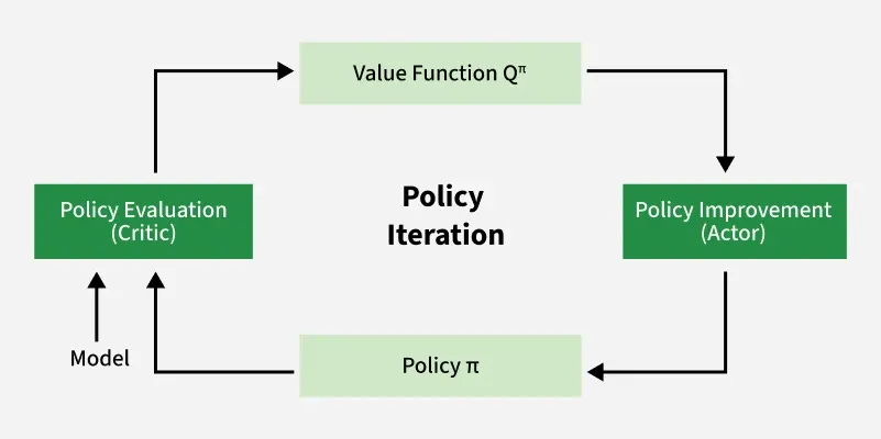
The powerful cycle of policy evaluation and policy improvement continues iteratively, driving the algorithm towards optimality. A fundamental and crucial characteristic of Policy Iteration is its guarantee of monotonic improvement. This means that each successive iteration is guaranteed to yield a policy that performs at least as well as, and frequently strictly better than, its predecessor in terms of expected long-term return. This consistent, non-decreasing enhancement of the policy's value at every step is a cornerstone of Policy Iteration's reliability and effectiveness.
Crucially, for finite state-action spaces, Policy Iteration is mathematically guaranteed to converge to an optimal policy within a finite number of steps. This explicit process of maintaining and continually refining the policy throughout its execution solidifies Policy Iteration as a robust and reliable method for discovering optimal control strategies.
Value Iteration (VI) offers a distinct and powerful approach to solving Markov Decision Processes (MDPs) by directly computing the optimal value function, V*(s). Unlike Policy Iteration, VI does not explicitly maintain or iteratively improve a policy throughout its process. Instead, it focuses solely on refining the value estimates for each state until they converge to their optimal values, from which the optimal policy can then be readily derived.
The algorithm begins by initializing an arbitrary value function, commonly setting V₀(s) = 0 for all states s. In each subsequent iteration k+1, the value of every state s is updated by considering the maximum expected return achievable from that state across all possible actions. This critical update rule is encapsulated by the Bellman Optimality Equation, which serves as the core iterative principle:
In this equation, R(s,a) represents the immediate reward received for taking action a in state s. The term γ Σ_{s'} P(s'|s,a)V_k(s') accounts for the discounted expected value of the next state, s', weighted by its transition probability P(s'|s,a) and evaluated using the current value function V_k. The entire expression inside the maximization, R(s,a) + γ Σ_{s'} P(s'|s,a)V_k(s'), effectively represents the Q-value of taking action a in state s and then proceeding optimally according to the current value function V_k. By selecting the action that maximizes this Q-value, Value Iteration iteratively builds up the optimal value function by considering increasingly longer planning horizons.
The guaranteed convergence of Value Iteration to a unique optimal value function is attributed to a fundamental mathematical property of the Bellman optimal operator: it is a contraction mapping. When the discount factor γ is less than 1, applying this operator repeatedly reduces the "distance" between successive value functions. This contraction property ensures that the sequence of value functions, V₀, V₁, V₂, ..., will converge to a single, unique fixed point, which is precisely the optimal value function V*(s). This theoretical soundness is crucial for Value Iteration, firmly establishing that the algorithm will arrive at the correct V*(s), without requiring formal proofs of this property during its conceptual application.
Once the value function V*(s) has converged to a stable state, the optimal policy π*(s) can be extracted directly. For each state s, the optimal policy simply dictates selecting the action a that maximizes the expected return, utilizing the converged optimal value function to evaluate future states:
It is an important distinction that while the value function itself monotonically converges to the optimal one in Value Iteration, the policy extracted at intermediate steps does not necessarily guarantee monotonic improvement. This contrasts with Policy Iteration, where policy improvement is a guaranteed step in each iteration.
Reinforcement Learning (RL) faces several significant challenges, which are central to the study of its mathematical foundations and practical applications:
1. Function Approximation
Classical Reinforcement Learning models often rely on tabular methods, which assume a finite number of states with stored values and policies. However, real-world applications like large-scale video games, autonomous driving, or complex robotic systems involve millions, billions, or even continuous state and action spaces. Directly representing or tabulating values and policies for such vast spaces is computationally intractable and memory-prohibitive. Function approximation, using parameterized functions like neural networks or linear models, approximates the value function (Q-values or state-values) or the policy directly. This allows RL algorithms to generalize from limited states to unseen ones, enabling scalability to environments with immense or continuous state-action spaces. The challenge then shifts from storing every state-action pair to learning and optimizing the parameters of these complex functions.
2. Partial Observability (POMDPs)
In many practical settings, an agent does not have complete or perfect information about the environment's true underlying state. Instead, it receives only limited, noisy, or incomplete observations. This condition introduces the significant challenge of partial observability, where the agent must infer the underlying true state from its incomplete observation history. For example, a robot navigating a cluttered room might only perceive its immediate vicinity through its sensors, rather than possessing a complete, global map of the entire room layout. Partially Observable Markov Decision Processes (POMDPs) are the formal mathematical framework used to model and study such scenarios. In POMDPs, agents cannot simply react to the current observation; they are required to maintain a belief distribution over possible true states, continuously updating this belief based on new observations and past actions. This belief state, rather than the true state, then guides the agent's decision-making, significantly increasing the complexity of policy derivation and learning.
3. Multi-Agent RL (MARL)
Multi-Agent Reinforcement Learning (MARL) addresses the complexity of RL when multiple agents interact in a shared environment. Agents can collaborate to achieve a common goal (e.g., robots) or compete (e.g., players in a game). Each agent’s perspective introduces dynamic and non-stationary environments, as the optimal policy depends on the evolving policies of other agents. This non-stationarity violates the core Markovian assumption in single-agent RL, where the environment’s dynamics are static. MARL research often draws upon game-theoretical perspectives to design algorithms and establish theoretical guarantees for these intricate multi-agent systems. Simple Markov policies may be insufficient; more sophisticated general policies that incorporate the full history of observations and actions are necessary to account for complex interdependencies and evolving behaviors.
4. Sample and Computational Efficiency
Two critical practical concerns in deploying Reinforcement Learning systems are sample efficiency and computational efficiency. Modern RL algorithms require millions to hundreds of millions of interactions with the environment to learn effective policies, which is prohibitively expensive, time-consuming, and potentially unsafe in real-world applications like training autonomous vehicles or operating physical robots. Reducing sample complexity is a primary goal in RL research, while computational efficiency addresses the substantial processing power required for training advanced RL models, especially those using deep neural networks. Iterative algorithms, based on principles from dynamic programming, mitigate high computational costs by avoiding expensive operations like large matrix inversions, especially in environments with vast state spaces. Balancing data requirements with practical constraints remains a significant hurdle for real-world RL deployment.
This guide explains the core principles of Reinforcement Learning, from agent-environment interactions and Markov Decision Processes to powerful control algorithms like Policy and Value Iteration. It explores how policies, value functions, and the discount factor define optimal strategies in complex state spaces through simulation. Despite challenges like function approximation, partial observability, and multi-agent interactions, understanding these foundational principles is crucial for designing intelligent systems that learn and adapt in dynamic environments.
Thank you so much for taking the time to read through my thoughts. This newsletter is a small space where I share my learnings and explorations in RL, Generative AI, and beyond as I continue to study and grow. If you found value here, I’d be honored if you subscribed and shared it with friends who might enjoy it too. Your feedback means the world to me, and I genuinely welcome both your kind words and constructive critiques.
With heartfelt gratitude,
Thank you for being part of Neuraforge!
Narasimha Karthik J