
Q-Learning, a groundbreaking breakthrough in reinforcement learning, offers a simple yet effective method for agents to learn optimal behavior through trial and error. This comprehensive guide delves into the theoretical underpinnings of Q-Learning, unraveling the mechanics of its renowned update rule. We will explore the fundamental “optimistic” nature of Q-Learning, contrasting it with its on-policy counterpart SARSA, and provide the core intuition necessary to grasp this essential temporal-difference control method.
To dissect algorithms like Q-Learning, we must first grasp the concept of off-policy learning. This paradigm allows an agent to learn about an optimal policy while following a different, more exploratory one. It separates the policy being learned from the policy used for generating experience, unlocking significant flexibility.
At the heart of off-policy learning are two distinct policies:
The Target Policy (π): The policy the agent aims to learn and perfect. In control problems, the goal is to make the target policy optimal. This is typically a greedy policy—one that deterministically selects the action with the highest estimated future reward.
The Behavior Policy (μ): The policy the agent actually uses to interact with the environment. To ensure the agent discovers optimal paths, the behavior policy must be exploratory, such as an ε-greedy policy that usually exploits the best-known action but occasionally chooses a random action.
Think of the target policy as a map of the theoretically fastest route. The behavior policy is you driving the car, occasionally taking a detour to see if it leads to a better shortcut. Off-policy learning updates your map (target policy) using insights from your detours (behavior policy).
This separation elegantly resolves the exploration-exploitation dilemma. The agent can use a "soft" behavior policy to gather a wide range of experiences, ensuring broad coverage of the state-action space. Meanwhile, the learning process uses this data to refine a separate, deterministic, and optimal target policy. This is valuable in real-world scenarios where an agent can learn an optimal policy by observing a human expert or analyzing historical data from a safer, previous policy.
With the foundation of off-policy learning established, we can turn to Q-Learning. Introduced by Chris Watkins in his 1989 PhD thesis, it was a breakthrough that presented a clear, provably convergent method for an agent to learn optimal behavior without a model of the environment's dynamics.
The central idea behind Q-Learning is to directly learn the optimal action-value function, q*. This function, q*(s, a), represents the maximum cumulative future reward an agent can expect by taking action a in state s and then following the optimal policy thereafter.
If an agent learns the true q* function, the optimal policy becomes trivial: in any state, select the action with the highest q-value. Remarkably, Q-Learning can learn q* regardless of the policy the agent follows to explore the environment.
Q-Learning is a model-free, off-policy, Temporal-Difference (TD) control method.
Model-Free: It learns directly from experience tuples of (state, action, reward, next_state), needing no predefined model of the environment.
Off-Policy: Its defining feature. The agent follows an exploratory behavior policy while its learning updates are based on the optimal greedy policy.
TD Control: It improves its estimates based on other learned estimates (bootstrapping) with the goal of finding an optimal policy (control).
At the core of Q-Learning is its powerful update rule, which blends immediate rewards with discounted, long-term value estimates. After taking action (At) in state (S_t) and observing the reward (R{t+1}) and next state (S_{t+1}), the agent updates its Q-value estimate:
Let's dissect its components:
Q(S_t, A_t): The current estimated value of taking action (A_t) in state (S_t).
α (Alpha): The learning rate (0 to 1), which dictates the weight given to new information.
γ (Gamma): The discount factor (0 to 1), determining the present value of future rewards.
R_{t+1}: The immediate reward received.
\max{a} Q(S{t+1}, a): The cornerstone of Q-Learning. It is the agent's estimate of the optimal future value achievable from the next state, (S_{t+1}). The agent considers all possible next actions ((a)) and selects the one corresponding to the maximum Q-value. This optimistic assumption is what makes the algorithm off-policy and drives it toward optimality.
We can reframe the equation to highlight its Temporal-Difference (TD) components. The TD Target is the value estimate our update is aiming for:
The TD Error measures the discrepancy between this new target and our old estimate:
The full update rule simply nudges the old Q-value towards the TD Target, with the size of the nudge scaled by the learning rate, (\alpha).
# Purpose: Updates a Q-table entry for a state-action pair using the Q-Learning formula.

def update_q_value(q_table, state, action, reward, next_state, alpha, gamma):
    """
    Updates the Q-value for a given state-action pair based on the observed
    reward and the estimated value of the next state.
    """
    # 1. Retrieve the current Q-value for the state-action pair.
    old_value = q_table[state, action]

    # 2. Determine the maximum Q-value for the next state, representing     # the optimal future value from that state (the 'max' operator).
    next_max = np.max(q_table[next_state])

    # 3. Calculate the TD Target: the reward plus the discounted optimal future value.
    td_target = reward + gamma * next_max

    # 4. Calculate the TD Error: the difference between the TD Target and our old Q-value.
    td_error = td_target - old_value

    # 5. Compute the new Q-value by adjusting the old value by a fraction (alpha) of the TD error.
    new_value = old_value + alpha * td_error

    # 6. Update the Q-table with the newly computed value.
    q_table[state, action] = new_value
To appreciate Q-Learning's design, contrast it with its on-policy counterpart, SARSA. The SARSA update rule is nearly identical, with one critical substitution:
The difference is how future value is estimated.
Q-Learning uses (\max{a} Q(S{t+1}, a)), assuming the agent will act greedily (optimally) from the next state. This max operator decouples the learned policy from the one being followed, making it off-policy. It learns the value of the optimal policy, regardless of which exploratory action it actually takes next.
SARSA uses (Q(S{t+1}, A{t+1})), the Q-value of the actual next action chosen by its behavior policy. This makes SARSA on-policy—it learns the value of the policy it is currently following, including its exploratory mistakes.
The Q-Learning algorithm is an iterative process. Within each episode, the agent repeats the following steps:
Observe the current state, (S_t).
Select an action (A_t) using an exploratory policy (e.g., ε-greedy).
Perform the action (A_t).
Receive a reward (R{t+1}) and new state (S{t+1}).
Update the Q-table using the experience tuple ((St, A_t, R{t+1}, S_{t+1})) and the update rule.
This loop repeats, with incremental adjustments guiding the Q-values toward their optimal counterparts. Q-Learning is proven to converge to q* provided two conditions are met: every state-action pair is visited infinitely often, and the learning rate (α) decreases appropriately over time.
The classic "Cliff Walking" environment perfectly illustrates the behavioral differences between Q-Learning and SARSA. An agent must navigate from a start to a goal, avoiding a cliff that gives a large negative reward. Every other step gives a small negative reward (-1), incentivizing the shortest path.
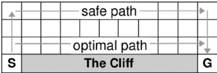
The optimal path runs directly alongside the cliff's edge, while a longer, safer path arcs far away from it.
SARSA, being on-policy, learns the value of its exploratory policy. Since a random exploratory step near the cliff is catastrophic, SARSA learns that the cliff-edge states are dangerous. It converges on the longer, safer path.
Q-Learning, being off-policy, uses the max operator to update its values based on a hypothetical, perfectly greedy future. It disregards the risk of an exploratory misstep and learns that the states along the cliff's edge lead to the highest reward. It converges on the optimal, but risky, path.
This algorithmic distinction creates a crucial trade-off:
During training (Online Performance): SARSA performs better. By quickly learning to avoid the cliff, it accumulates higher, more stable rewards per episode. Q-Learning performs poorly, as its agent frequently falls off the cliff while exploring the optimal path.
After training (Final Policy): When exploration is turned off, Q-Learning's final policy is truly optimal—it executes the shortest route. SARSA's final policy is sub-optimal, executing the longer, safer route it learned during its cautious exploration.
This highlights a key question for practitioners: is it more important to maximize performance during learning, or to discover the absolute best policy, irrespective of exploratory costs?
Q-Learning is an optimistic learner. It updates its values assuming it will act optimally from the next step onward, even as its current self makes mistakes. SARSA is a more conservative learner, grounding its values in the reality of its own error-prone behavior. This makes SARSA a safer choice in applications where exploratory mistakes are costly or dangerous.
Q-Learning remains a foundational algorithm in reinforcement learning due to its elegant, off-policy approach. By leveraging the max operator in its update rule, it decouples learning from behavior, allowing it to identify the optimal policy even while exploring sub-optimally. Understanding this optimistic strategy and its trade-offs is key to solving control problems and serves as the perfect stepping stone to grasping more advanced methods like Deep Q-Networks.
Thank you for reading my thoughts. This newsletter is a humble space where I share my journey in RL, Generative AI, and beyond. If you find value here, I’d be grateful if you subscribed and shared it with friends. Your feedback, both kind and constructive, helps me grow.
With gratitude,
Narasimha Karthik J